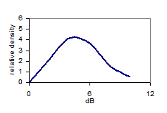
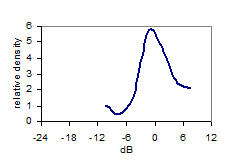
Fig 11,top: FR normalized to band average (0dB), in 25Hz wide band centered at 125Hz; Bottom: Level distribution in band; SD=4dB.

Stochastic nature of room acoustics 1

The Schroeder frequency:

 f_c  ~2000·(T/V)^0.5

This is an akuTEK article by M Skålevik           www.akutek.info main page   article site index page

(1)

www.akutek.info

Average spacing vs Quantization of level

N = 4p / 3·( f / c)³·V

Number of modes below frequency f (Hz):

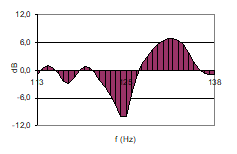
Fig 8: FR in a 90m³ room, f_c ~170Hz

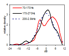
Fig 9: FR level distribution

Fig 10: Distribution above and below f_c

The data in Table 11 does not indicate that the level distribution in the 70-170Hz region is of a different nature than in the 200Hz-2.8kHz region. We conclude that in this case, from the study of peak spacing and level distribution, the Schroeder Frequency does not represent an observable cross-over frequency between two significantly different frequency regions.

We shall need more data to continue this investigation, searching for an observable cross-over frequency.

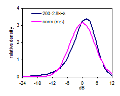
First we shall study the level distribution (dark blue curve, Fig 9) of the FR in the 90 cubic meter room, above the Schroeder Frequency (200Hz to 2.8kHz), along with a normal distribution having the same average and standard deviation as the FR. The bell-shape reflects the Gaussian properties, confirming Schroeder’s theory. The FR in this region can be considered stochastic and we shall use its distribution as reference in the following low frequency analysis. Note the asymmetry (skewness= –1.1dB) of the level distribution as must be expected since the dB-scale goes from -∞ to 6dB as sound pressure goes from 0 to 2 times the reference pressure at 0dB. The level distribution curve deviates 9% from the normal distribution curve (RMS deviation). 90% of the FR levels are between –9 and +7dB.

Now turning to the region below the Schroeder Frequency f_c (Fig 10), the distribution curves (red curve 70-170Hz) seem to deviate considerably from the curve of the reference region 200-2.8k Hz (dotted curve). The deviation (RMS) is 17% in the 70-170Hz region, which is more than in the 170-270Hz region. However, the deviation in the 270-370Hz region is even greater (18%), meaning that the deviation below the Schroeder Frequency is not significant.

Standard deviation is 5.4Hz in the 70-170Hz region. Neither this or the 5% and 95% percentiles show significant differences from the values above the Schroeder Frequency. Table 11 below summarize the key properties of the different frequency regions.

Case study—Level distribution

Case study—Observed cross-over

In general, we want to support theory by observations. In particular, we want to support the theoretical cross-over frequency suggested by Schroeder by results with proper statistical significance. Procedure in steps as follows:

Search after an observable cross-over frequency

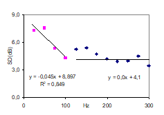
Step 6 in the procedure above has resulted in an observed cross-over frequency, detected by a best fit line method, at 107Hz, which is equal to 0.63 times the Schroeder Frequency of the room.

In further work, the result will be compared with measurements from other rooms, and discussed in relation to possible theoretical explanations.

For a start, figure 15 presents a case with no detectable crossover, for a single point in a different room than the case above. The volume of the room is 50m³ and the reverberation time in the possible crossover region is 0.39s.

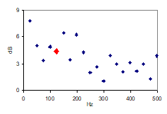
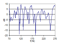
Fig 12: SD(dB) in 25Hz bands from one FR. Red dot indicates the 125Hz band.

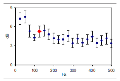
Fig 13, top: SD (dB) in 25Hz bands, room average and 5% confidence intervals from 23 FRs in the 125Hz band (red dot). Bottom: Spatial distribution of SD’s in the 125Hz band

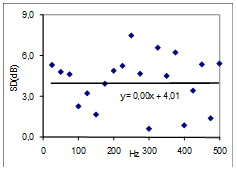
Fig 14: Best fit lines for two frequency regions cross at f=107Hz

Fig 15: Similar to Fig 14, but a different room (V=50m³, T=0.39s), single measurement, no detectable cross over.

Case study, observed Cross-Over-Frequency, conclusion

Discussion

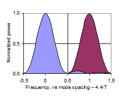
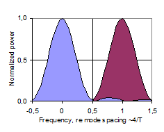
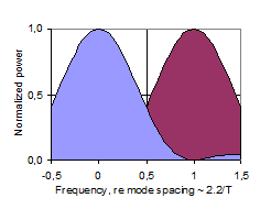
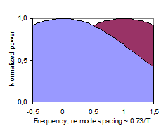
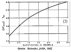
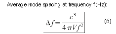
In this theoretical discussion of significant regions of the frequency response, the frequency region above the Schroeder Frequency, for which Schroeder’s stochastic theory is valid (Gaussian level distribution, 4/T average spacing between maxima, etc.), will be referred to as the High Frequency (or HF) region. Below the HF region there is a transition region, below which the Low Frequency (LF) region is of a nature that is significantly different from the HF region.

Historically, the Schroeder Frequency has evolved as a limit above which the frequency response is likely to be dominated by stochastic processes. In 1954, Schroeder suggested a criteria of a 10-fold modal overlap on average, resulting in a critical frequency of 4000·(T/V)^0.5. In his 1962 paper, he refers to several measurement reports indicating that the critical frequency may be as low as the current one (1), corresponding to an average 3-fold modal overlap, fig 16. However, this does not in it self exclude the possibility of stochastic nature at even lower frequencies. While the Schroeder Frequency serves well as a lower limit for the HF region, it is less suitable as a higher limit for the LF  region. The latter is expected to be dominated by average spacing between maxima that is wider than the modal bandwidth.

A possible two-sided cross-over frequency could be the frequency having an average mode spacing equal to the average modal bandwidth ~2.2/T, fig 17, which could be the center of a more or less wide and symmetrical transition region. However, below this cross-over frequency the average mode spacing is Df > 2.2/T, and in particular there will occur the mode spacing Df ~4/T, fig 18, which according to Schroeder is a characteristic feature of the HF region, contradicting this cross-over frequency candidate. In some cases it will in fact be impossible to distinguish an observation of mode spacing equal to 4/T and a maxima spacing equal to 4/T. This implies that in the Low Frequency region, the mode spacing must be on average wider than 4/T. Further, when average modal spacing is more than two times the modal bandwidth, Df >4.4/T, fig 19, more than 50% of the frequency response will depend on direct energy from the source, referred to below as <50% modal density. Corresponding wavelengths will be larger than the square root of the room absorption area, l>A^0.5.

We may conclude that the transition region can be defined by several mode spacing criteria, with corresponding frequencies computed from (6). Moreover, the upper frequency limit of the region in which the near-field of a sound source is significantly influenced by reverberant sound pressure, i.e. the near-field extends into the reverberant field (kr_c < 1), falls in the very middle of this transition region. A summary is given in Table 20 below. Corresponding average mode spacing and modal overlap is illustrated in fig’s 16-19.

Continued in Part 2

First published 19.03.2009, latest change 12.10.2012

Related:

Tonal response in rooms (Microstructure of room acoustic FR), a presentation by M Skålevik
Schroeder Frequency Revisited  FA 2011 presentation  29.06.2011
Schroeder Frequency Revisited  (Forum Acusticum 2011 paper) 17.04.2011

Go to www.akutek.info main page     Go to article site index page

Fig’s 16-19: Illustration of two adjacent modes with mode spacing normalized to unity. Degree  of modal overlap and density decreasing from top to bottom, with 3-fold overlap in (16) to 50% modal density in (19).

Share this:

HOME

INDEX