akutek.info

The www center for search, research and free sharing in acoustics

Binaural localization

2014-11-21 Localization of binaural pure tone, invitation: “Listen to each of the examples, by clicking on their respective link, labeled by letter A to N.  All examples are of duration 6s, but in most players you will be able to end and start another by just clicking on another link whenever you like. Headphones required, and you should start by doing the 3 headphone tests below.

Where is the sound source located, on a scale from left to right?

During listening with headphones, please assign to each example A thru N the apparent lateral position you perceive by checking the appropriate box. If you feel that some of the examples are not point sources, please describe in the comments box, referring to the example letter.

Make sure to do the headphones and channel check first (top of web page)

Feel free to repeat and use as much time as you like. Please click the “Finished” button when finished.“

Headphone test 1, sound in Left channel only:    http://akutek.info/wav/sine440HzLeftonly.mp3

Headphone test 2, sound in Right channel only: http://akutek.info/wav/sine440HzRigthonly.mp3

Headphone test 3, sound image should be centered (adjust L-R balance): http://akutek.info/wav/sine440Hz.mp3

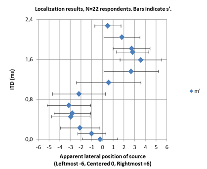
2014-12-02 Results after N=22 responses are given in the table below. Description of test object: Binaural 440Hz pure tone with lag in Right channel. Columns are Interaural Time Differences ITD in milliseconds (ms) and absolute radians (rad), relative phase lag of Left channel in % of period T (e.g  absolute lag 100%T = relative lag 0%T), average of 22 responses m’, standard deviation s’, and interval of 95% confidence around m’, c’. Common unit of m’, s’ and c’ equals one step in the assessment scale ranging from –6 (Leftmost) to +6 (Rightmost), with 0 denoting centered localization of sound image. Average s’ is 1.9 and average c’ is 0.79. Sound level difference between ears are assumed to be zero (ILD=0dB) since all respondents confirmed the reference sound in Test 3 to be centered.

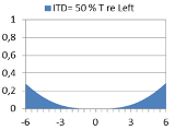
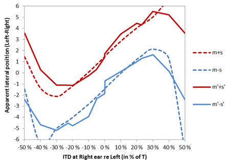
Comments to result, Figure 1: In humans, ITD=0.6-0.7 are more rare, and 0.8ms is usually taken as the biggest natural ITD, limited by size of the human head and position of ears. Maximum lead=0.8ms at Left ear would occur with a source directly to the left. For ITD greater than 0.8s, ambiguous positions must be expected from all respondents. Such ITDs can not in nature be caused by a single point source, but rather by a secondary source or an image source (reflected sound).

 

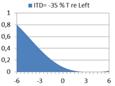
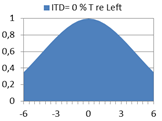
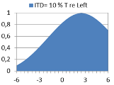
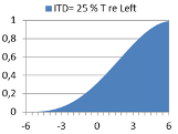
What would a binaural model predict? Below are diagrams showing  predicted probability of lateral localization. The model is a simple version of Jeffress’ Coincidence model, assuming a half-rectified signal propagating along a delay line from each ear, calculating inter-aural cross-correlation (IACC) at so-called coincidence cells where the signals meet along their repective delay lines. We shall here interpret the distribution of IACC over the lateral scale from left to right as the probability of perceived  localization of the source. For each ITD expressed as phase difference in % of a period T, a characteristic distribution is calculated, as presented in examples of diagrams below. In each distribution, the mean value m can be interpreted as the average estimate for the lateral position, while the standard deviation s describes the uncertainty in the estimate of m. The diagram with phase difference 50% of T (Left and Right perfectly out of phase) illustrates a special kind of ambiguity which some perceive as a split sound image - apparently one source at the Left and one at the Right. In a diagram further below, the predicted m and s are compared with the m’ and s’ from the statistical results of the listening test above.

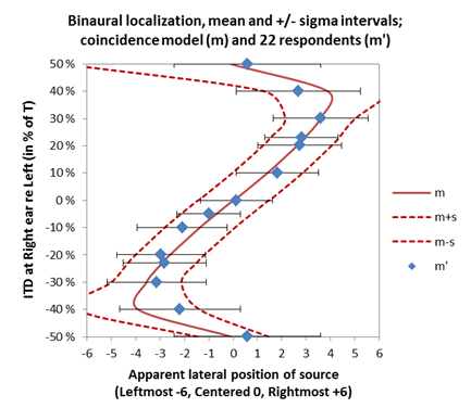
Figure 3, above:  Localization result statistics (m’ and +/-s’ intervals) after 22 respondents, and  predicted localization probability (m and +/-s intervals) from the coincidence model, see text.  Vertical axis is phase at Right ear relative to Left ear, in % of a period T. Horizontal axis is lateral position.

Figure 4, above:  Localization distribution in terms of +/- sigma intervals around mean. Solid curves indicate distribution after listening test [m’-s’, m’+s’] after 22 respondents; Dashed curves indicate probability distribution [m-s,m+s] predicted with the coinsidence model, see text. Horizontal axis is phase at Right ear relative to Left ear, in % of a period T. Vertical axis is lateral position.
Comment:  In most humans, a 440Hz point source in free field will seldom create phase differences larger than +/-25% of T. The diagram shows that listening tests outside this interval deviates more from predictions than the smaller, ”natural”, phase differences.

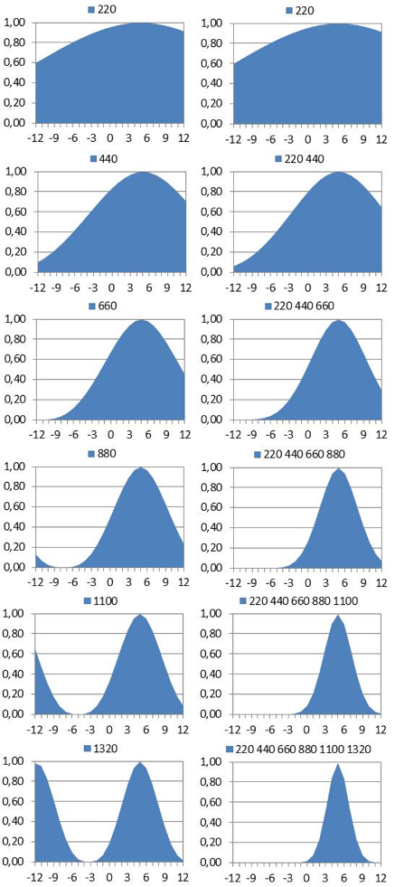
More cues—more accuracy in source localization: The 440Hz pure tone above provides one single localization cue only. As can be seen in figures above, this single cue has considerable uncertainty. However, sound sources are usually far more complex than the pure tone case, and in many complex cases binaural hearing rely on two sets of cues - the ITD cues (as applied in the case above) and the ILD cues (Inter-aural level difference occuring when sources at one side of the head casts sound shadows on the ear at the far side of the head). Both the ITD cues and the ILD cues are numerous, as they come in families of critical frequency bands. ITD cues are most important in the bands below 1.5kHz, and the ILD cues are most important in the bands above 1.5kHz. Sources emitting transients or periodic sounds with many partials are examples of sources that provide many cues. Compared to single cue in the ITD of the pure tone tone above, each extra cue would potentially reduce the uncertainty in localization of the source. Bearing in mind that each cue has a localization probability function like the one for the 440Hz tone (Figure 2a-e, above), the resulting probability could be predicted by multiplying the probability functions of each cue. The product of probabilities would typically produce a profile that is more narrow than those from the single cue in Figure 2a-e, thus demonstrating the improved accuracy of the increased number of cues, see example in Figure 5.

Figure 5, right: Predicted localization of a sound source becomes more accurate for every partial that is added.  The diagrams in the left  column are localization probabilities of each separate partial (pure tones) 220Hz, 440Hz, ... Each partial is a cue. Note the growing ambiguity in 880, 1100 and 1320Hz. The diagrams in the right column are products of the probability functions as partials are added one by one. E.g., third from the top is the diagram of the product of probablity functions of the three first partials partials 220Hz, 440Hz and 660Hz. Note that the ambiguities seen in separate partials 880-1320Hz are eliminated, and that even the 1320Hz cue provides improved accuracy, despite its peak at far left (-12).
ITD = 10 samples at rate 44.1kHz = 0.23ms = 5% of T at 220Hz = T/4 at 1100Hz. This compares to an azimuth of about 25 degrees to the right, depending on head size and shape.  For simplicity we shall ignore non-zero ILD’s toward higher frequencies could provide additional cues.
This model has 25 coincidence cells representing positions from –12 to +12 on the lateral scale, i.e. from left to right. Each step corresponds to a time difference between each coincidence cell of one sample at rate 44.1kHz.

How weak can a cue be and still add to accuracy? The answer is, if a cue gets weaker compared to any masking effects (noise, spectral masking, temporal masking, etc.) , the inter-aural cross-correlation IACC will get weaker and a less prominent peak will be seen in the profile from the probability function. Ultimately the profile would be flat and the cue would not add to accuracy.

Figure 1

Litterature: Binaural hearing

J Blauert: Spatial Hearing: The Psychophysics of Human Sound Localization

J Blauert (Editor): The Technology of Binaural Listening

J Blauert: Binaural Models and their Technological Application 

Howard and Angus: Acoustics and Psychoacoustics

Fastl and Zwicker: Psychoacoustics. Facts and Models

Floyd Toole: Sound Reproduction: The Acoustics and Psychoacoustics of Loudspeakers and Rooms

Gilkey and Anderson: Binaural and Spatial Hearing - in real and virtual environments

M Schröder: Comparative Study of European concert halls: correlation of subjective preference with geometric and acoustic parameters (problems with URL has been reported)

Sue Harding Binaural Processing

Stern, Wang, Brown Binaural Sound Localization

A Oxenham (Lecture) Binaural hearing   

Sound localization (wikipedia)

R.Y Litovsky: Binaural Hearing (external site) 

J Breebaart: Sound Binaural processing model based on contralateral inhibition.I. Model structure

Sound Binaural processing model based on contralateral inhibition.II. Dependence on temporal parameters

Sound Binaural processing model based on contralateral inhibition.III. Dependence on temporal parameters

Misc. Authors: Localization of  sound sources (external site) 

  

Ambiguous cues: Localization cues can be ambiguous in several ways.

Different ITDs can produce similar phase difference, thus the same localization estimate, see Figure 1.

ITDs longer than 0.6-0.8s cannot be caused by a single point source in free field, given human head size, but can be learnt to be cues of source complexity or cues about the environment (reflected sound) of source and/or receiver. 

Cone of confusion : Different source azimuth can produce the same ITDs.

ITD=T/2 can produce split sound image, apparently one source at each side.  

on site